
|

By Pops
TopCoder Member
Introduction
In a nod to the Intel Multi-Threading Competition Series, I've decided to deviate a bit from the design pattern series and explore a few parallel programming patterns. Similar to design work, parallel programming has a number of patterns that can help a person recognize trends in data processing and to efficiently process those trends in a multi-threaded environment. The first pattern we will explore is the WaveFront. This pattern describes a set of strategies to efficiently process data over multiple threads when the flow of processing resembles a 'wave' (more on that later). This pattern is a good candidate where you have dynamic programming or any divide and conquer type of scheme that can become more efficient when processed over multiple threads.
Levenshtein distance
To understand this pattern, let's look at a common algorithm that involves some dynamic programming: Levenshtein distance. This algorithm is used to determine the edit distance between two strings. An edit distance is defined as the minimal number of character insertions, deletions or substitutions to transform one string (called the source string) into another (called the target string). Side note: this is also a good data entry algorithm to provide a data entry typist with good alternatives if the item they type is a misspelled value (like vendor or supplier names).
The distance between a source string of "bottomcoder" and a target string "topcoder" would be 4 because you would drop the initial "b", "o", "t" and change the "m" to a "p" (4 changes).
The algorithm works by laying out the strings in a grid and assigning the first row/column as follows:
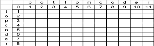
You then iterate the grid through the grid assigning each cell the following value (where r is the current row and c is the current column:
cost = if (d[r,0] == d[0,c]) then 0 otherwise 1
d[r,c] = min(d[r-1,c] + 1,
             min(d[r,c-1] + 1, d[r-1,c-1] + cost))
Basically this is saying that the cell's value is based on the minimum cost of changing the upper value, changing the lower value or potentially changing the current value. A filled out grid looks like:
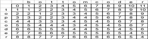
The final cell value represents the edit distance – in this case 4.
Back to the WaveFront Pattern - Recognition
If we study how the data flows from cell to cell, we'll see that a cell will flow the data to the right, to the bottom right and to the bottom. On an aggregate scale we will see:
The flow of information describes how and when each cell can process the information. Once cell 1 has completed – it flows it's information to the right, right bottom and bottom. Cells 2 can then be processed (note that cell 3 [that is to the bottom right of cell 1] cannot be processed until cells 2 have processed). Once cells 2 flow their information, cells 3 can then be processed and so on. This type of processing resembles a processing wave and provides us with the recognition that the WaveFront pattern strategies may apply to our algorithm.
WaveFront Strategies
Now that we have recognized the pattern, let's discuss the strategies that can enable us to take advantage of multiple threads. Any parallel pattern strategy attempts to minimize the communication between threads (i.e. the synchronization between threads to communicate the data), to minimize the idle time for any given thread (i.e. we want to keep our threads consistently busy) and to provide an even load balancing across each thread (i.e. so each thread does the same amount of work). If we achieve those three goals, then data was processed in as efficient a manner as possible.Fixed Block Based Strategy
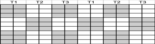
This strategy simply divides the rows and columns by the number of threads and allocates each thread that block of information to work on. If we have 3 threads we will be using, we could divide a 12x9 grid into blocks of 4x3s and assign the threads as shown here:
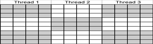
Thread 1 will process the first block (i.e. the first wave). When that is completed, the second wave is processed by both thread 1 and thread 2 (the white cells to the right and bottom of the first wave). By the third wave, thread 3 has joined our processing.
The advantages of this approach are that the communication between each thread is minimized (i.e. a lot of cells are processed without having to communicate to other threads) and that the balance of work is evenly spread across threads (each thread is responsible for 3 blocks and each block processes the same amount of information).
The disadvantage of this approach is that idle time is not minimized and in fact, is quite prevalent. Thread 3 is idle until wave 3 is processed. Thread 1 become idle after the third wave.
This strategy is the simplest to implement and would be an ideal approach if the communication time between threads is more expensive then the cost of having threads that are idle.
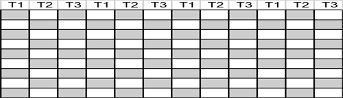
Cyclical Fixed Block Based Strategy
As shown above, the biggest disadvantage is in the idle time of threads. Choosing a cyclical fixed block strategy pattern can help alleviate this disadvantage by balancing the load, per wave, by cycling over the various threads by using smaller block sizes. An example would be to drop the block size down to a 2x3 block and then cycle the threads over the blocks:
As you can see, this helps to minimize the idle time by allowing each of the threads to participate in more waves and on smaller blocks. However, there is a tradeoff in the inter-thread communication because less work per block can be done independent of other threads.
If the cost of the communication is extremely low and idle time cost is high, you can even choose 1x1 blocks (as shown below) that will minimize the idle time at the cost of maximizing communication.
The cyclical block strategy provides a nice balance between the cost of communication and the cost of idle time while the programmer can play with the block sizes to provide an optimal combination.
Variable Cyclical Block Based Strategy
The above strategies work well because each cell has the same processing time involved (evaluating 3 other cells to determine this cell) and would be ideal for the Levenshtein algorithm or any other fixed processing based algorithm. However, there are many times when the processing time can vary cell by cell. Consider the following algorithm:
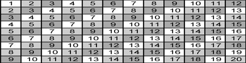
d[r,c] = min(sum(d[0…r-1,c]), sum(d[r,0…c-1]))This algorithm specifies each cell processing the cells before it and the cell's processing time will increase the farther away from the origin the cell is. Please look at the following for a demonstration of this:
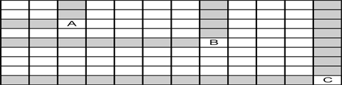
You can see that cell A needs the values from 4 other cells. Cell B will process 11 other values and cell C will need the most at 19 values. So the time spent calculating the cell's value is skewed in the direction of the wave itself. If we were to choose fixed block sizes, the balancing of load between the threads will be uneven because the fixed block size does not take into account the processing size of each block and each block will become more expensive than the last.
The solution would use variable sized blocks. In the example below, we process the first three waves using a large block size and reduce the block size as the processing cost increases:
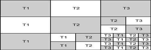
This allows us to balance the load over all the calculations yet still gain the advantages of minimizing communication needs.
Conclusion
The WaveFront pattern is a good introduction to the parallel patterns that is fairly easy to implement, understand and is more generally useful (and is one of the more simplistic patterns). Like all patterns, you need to understand the flow of data and processing, recognize it and then apply the appropriate strategy to deal with it.
As a last word, good luck in the Intel Multi-Threading Competition Series!